Incorporating Local Road Grades and Times-of-Day Traffic into Vehicle Specific Power Profiling for Urban Freeway Vehicle Emission Estimation - Juniper Publishers

 Juniper Publishers- Open Access Journal of Environmental Sciences & Natural Resources

Incorporating Local Road Grades and Times-of-Day Traffic into Vehicle Specific Power Profiling for Urban Freeway Vehicle Emission Estimation

Authored by Heng Wei

Abstract

Vehicle Specific Power (VSP) is conventionally defined to represent the instantaneous vehicle engine power. It has been widely utilized that the impact of vehicle operating conditions on emission and energy consumption estimation is associated with vehicle speed, roadway grade and vehicle acceleration or deceleration on the basis of the second-by-second vehicle operation. VSP is hence incorporated as a key contributing factor into the vehicle emission models in MOVES. For practical application, however, it is always cumbersome to accurately profile VSP distribution by collecting and using localized grade and times-of-day traffic data. Therefore, it is necessary to clarify the impacts of these factors on highway vehicle emission estimation. This paper presents a study in which previous studies are extended by deeply investigating the characteristics of VSP distributions and their impacts due to varying freeway grades, as well as time-of-day traffic factors.

Statistical distribution models with a scope of bins is identified through a goodness of fit testing approach by using the Global Positioning System (GPS) data collected from the interstate freeway I-75 segments in the Cincinnati area. The data was collected at a selected length of 30 km urban freeway for AM, PM and Mid-day periods. The datasets representing the vehicle operating conditions for the VSP calculation were then extracted from the GPS trajectory data. The results of distribution fitting show that the Wake by distribution is able to capture most distribution characteristics of VSP at all grade bins under a higher speed variation condition, and the generalized logistic distribution fits the sample data better at grade bins between -4% and 4%when the speed variation is lower. In addition, the speed variation lying behind the times-of-day differences is also identified to be a contributing factor of urban freeway VSP distribution. The enhanced understanding and modelling of VSP distribution by roadway grade provided by the study can facilitate the preparation of MOVES vehicle operating mode distribution inputs.

Keywords: Vehicle Specific Power Distribution; Second-By-Second GPS data

Abbreviations: VSP: Vehicle Specific Power; GPS: Global Positioning System; SIP: State Implementation Plan; U.S. EPA: United States Environmental Protection Agency; ISSRC: International Sustainable Systems Research Centre; HDOP: High Horizontal Dilution of Precision; MLE: Maximum Likelihood Estimates; K-S: Kolmogorov-Smirnov; HDV: Heavy Duty Vehicle; LDV: Light Duty Vehicles; BRT: Bus Rapid Transit

Introduction

Global Positioning System (GPS) data collected locally, providing high-temporal resolution (e.g. second-by-second) speed, acceleration or deceleration driving cycles, enables modelling the impact of vehicle operation conditions on emission and energy consumption with Vehicle Specific Power (VSP) for local projects. MOVES, developed by the United States Environmental Protection Agency (U.S. EPA), are used to estimate emissions for various mobile emission sources and allow multiple scale analysis such as emission budgeting of State Implementation Plan (SIP) and transportation conformity purposes [1]. In applying the MOVES model, it is required to convert traffic inputs into the VSP distribution, i.e., operating mode distribution [2], to satisfy the need of generating an operating mode distribution for MOVES for maximizing its capacity to accurately reflect real-world emissions.

It is critical to recognize the similarities and differences of engine instantaneous power distributions on a given roadway. There has been a substantial body of research on VSP distributions among roadways [3,4], vehicles [5], and vehicle speeds [6]. In addition to the speed and acceleration, the grade is another critical factor for estimating VSP However, this factor has been usually overlooked and always assumed to be zero in many previous studies. In such cases, freeways located in hilly terrains of urban area cannot be realistically represented and modelled. As a consequence, the calculated VSP may be less representative of the urban traffic fleet and then become insufficient to estimate the characterized emissions. To facilitate the preparation of the MOVES vehicle operating mode distribution inputs, an enhanced understanding and modelling of the VSP distribution within the road grade incorporated become indispensable. This paper presents a study in which previous studies are extended by investigating the characteristics of VSP distributions and their impacts due to varying freeway grades, as well as time-of-day factors.

Statistical distribution models with a scope of bins is identified through a goodness of fit testing approach by using the GPS data collected from the interstate freeway segments in Cincinnati area. In the rest of the paper, firstly, the literature reviews on the VSP profiling study is presented followed by the introduction of the data used in this study. Then, the methodology regarding VSP calculation and VSP binning is introduced, and the case study results of urban freeway segments in Cincinnati urban area are presented. Next, sample distribution fitting results for basic freeway segments are illustrated. Finally, the paper is summarized with conclusions and recommendations for further research.

Literature Review

VSP derived from second-by-second vehicle activities is critical to the on-road emission modelling. Besides that, microscopic simulation outputs can also be used to generate inputs for VSP distribution and MOVES. In the simulation based dynamic traffic assignment model for project level emissions analyses developed by [7], the operating mode distribution based on VSP distribution is calculated and used as MOVES model inputs. The procedure of deriving MOVES operating mode distribution using VISSIM simulation results was introduced by [8,9] pointed out that for vehicle emission estimation, the use of VSP distribution to calibrate micro-simulation model is more reasonable than using conventional approach [10] proved that there is direct physical interpretation of the distribution characteristics of VSP and it has well statistical relations with on-road vehicle emissions [11] investigated VSP distributions and emission rates for five driving cycles from mild to aggressive [12] concluded that there were significant similarities when speed profiles of different roadway facility types are grouped by average link speed.

Especially, where a mean speed is between 20 and 30 km/h, VSP distributions are found to be very identical. In [13] study, GPS and PEMS data was collected to investigate correlations between VSP and pollutants. It has been suggested that higher VSP values relate to higher emissions of Nitrogen Oxidizes, Hydro-Carbon, Carbon Dioxide, and Carbon Monoxide [14,15]. To determine driving patters of on-road vehicles and supported the development of the IVE model, VSP distribution patterns for Nairobi, Santiago and Sao Paulo have been included in the International Sustainable Systems Research Centre (ISSRC) funded handbook of air quality management project by [16]. A study by [4] investigated VSP distribution among urban restricted access roadways and suggested that the distribution of VSP at various speed bins follow normal distribution. Based on this distribution assumption, the mean and standard deviation of VSP are modelled by using regression techniques.

The VSP distributions on the low speed (less than 20 km/h) segments by using the same methodology were investigated in a later study by the same authors. VSP distributions for every speed from 1-20 km/h are calculated and a quadratic relationship between VSP fraction and the VSP bin number was observed [5] concluded that normal distribution is most likely the case for travel speed lower than 90 km/h for both Heavy Duty Vehicles (HDV) and Light Duty Vehicles (LDV). Besides, default operating mode distribution patterns in MOVES are very similar to their experimental data. Through a study on the VSP based driving cycles of regular and express bus line and Bus Rapid Transit (BRT), [6] concluded that the distribution of VSP may shifts to the right and does not follow the normal distribution when the average speed is greater than 25 km/h. However, in most of previous studies, the grade as one of the most critical contributing factors of VSP has been overlooked. There is an essential need of fill the gap. To extend previous work on freeway VSP distribution, the paper calculates the second-by-second distances travelled and generates the freeway grades for the VSP calculation and then fits the VSP samples into a grade-specific distribution. The grade- specific VSP distribution should allow a better comprehension of impacts of traffic operations on emissions.

Data

To fulfil the identified gap, a group of freeway segments from the Interstate Freeway 71 (I-71) within the Cincinnati urban area were targeted as the study site. The total length of the selected freeway segments is about 60 km for a round trip. To measure travel time reliability, the second-by-second GPS data was collected by group of students. Vehicles used in this data collection were chosen completely randomly. The data collection period covers AM peak hours from 7:00 AM to 9:00 AM, PM peak hours from 4:30 PM to 6:30 PM and Mid-day from 11:30 AM to 1:30 PM. A total of 38 trips were made from January 24th to April 20th, 2012. For the AM perk hours, 36,503 data points were collected, 27,931 data points for Mid-day and 42,624 for PM peak hours. There were approximately 110,000 records of data collected on the 30 km Interstate freeway. To remove invalid data from satellite signal lose, a data filter with high horizontal dilution of precision (HDOP) higher than 4 and low number of satellites (NSAT) less than 4 [17] was applied. After the data filtering, 97,491 records were used in the VSP calculation.

VSP and Binning

The mathematical presentation of VSP, first developed by [18], is calculated by dividing the summation of acceleration, rolling resistance, engine load against aerodynamic drag, and the kinetic and potential energies of the vehicle by the mass of the vehicle. In practice, a generic set of coefficients values estimating VSP for a typical light duty fleet is applied as a useful basis for characterization [19]. The VSP values for light duty vehicles are calculated by the following equation:

Where, v is vehicle speed (m/s); a is vehicle acceleration/ deceleration rate (m/s²); grade is vehicle vertical rise divided by the horizontal run (%). The horizontal run is measured by using the haversine formula in which it is assumed that the trajectory travelled between two consecutive points is a straight line in calculating shortest distance over the earth's surface. Even at small distances, the great circle distance between two points remains particularly well-conditioned for numerical computation [20].

Where, Lat is Latitude; Long is Longitude; R is radius of earth (mean = 6,371 km). Calculations of grade and VSP are implemented in R.A minimum interval of 1 kw/ton is used to avoid any bias, which can be incorporated in the binning and to draw out the quantitative relations between the VSP distribution and the grade by using the smallest bin possible. The VSP ranges from -20 to 20 kw/ton based on the data collected from urban areas, e.g. Beijing is used in many previous studies [5,14]. While, the VSP range from less than zero up to 30 plus is used in MOVES model to capture the VSP on U.S. highways [21]. Using the dataset collected at the study site, 98.32% of the calculated VSP values using Equation (1) falls into the range of -30 to 45 kw/ton. Therefore, VSP bins from -30 to 45 kw/ton are used in the paper.

The binning is presented as Equation (4) shows:

VSP Distribution Fitting and Goodness of Fit Testing

A. Freeway Grade Distribution

The freeway grade at the study site was calculated with Equation (2) and (3).A total of 92,914 grade data points is obtained. The samples collected shows that 92.35% grade data falls into the range from -10% and 10%. The distribution of freeway grade distributions at two percent interval is presented in Table 1. It is noticed that merely the grade between any data points equals to zero, which means the zero grade is rarely the case for urban interstate freeways in some of the U.S. metropolitan areas. Therefore, in VSP based emission and energy consumption modelling, the grade is an influential factor cannot be ignored. In the table, the distribution of freeway grades for the AM, PM peak and Mid-day is listed as well. In the collected data, 90.15% AM, .97.3% Mid-day and 92.01% PM data falls into a grade range of -6% to 6%. The distribution near perfectly follows bell-curves of normal distribution. As grade values are mostly within the range of -6% to 6%, it can be concluded that the selection of grade bins from -10% to 10% is justified and the range can well represent the real-world condition.

B. Candidate Distributions

From Table 1, the VSP distribution among the 12 grade bins seemed to be well presented by a normal distribution. However, Q-Q plots suggest that the sample tails are not quite following the normal distribution since they are rarely straight. In addition, there are peaks in almost all the histograms. A distribution fitting based on Q-Q plots and above observed distribution characteristics in Table 1 is necessary. Two distributions, generalized logistic distribution and Wake by distribution, are observed that can fit the data well. The Percentile-Percentile (P-P) plots comparing middles of sample distribution and model distribution are made. Afterwards, the goodness of fit testing for each of grade and time specific VSP datasets is determined based on the Kolmogorov- Smirnov (K-S) test.

The probability density function of generalized logistic distribution is given as Equation (5):

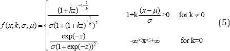
Where,, k is the shape parameter; σ is the scale parameter (σ>0); μ is the location parameter. The probability density function of Wake by distribution is described as Equation (6):

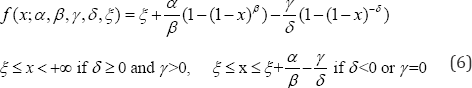
Where β,γ and δ are shape parameters; ξ and a are location parameters. To eliminate any bias brought from the negative values of the VSP, a linear transformation is performed so that the sample distributions have a range of positive values yet the distributions remain unchanged.

Where, VSP is the transformed VSP and VSPx is the original VSP value.

C. Parameter Estimation and Good of Fit Testing

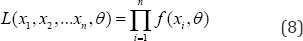
The maximum likelihood method is used to estimate parameters. It maximizes the likelihood of a set of parameter values from the probability model to observed outcomes through an iterative procedure. The values of sets of parameters that maximize the sample likelihood are called Maximum Likelihood Estimates (MLE). The function is defined as:

Where, 0 is the likelihood function. The goodness of fit testing using the Kolmogorov-Smirnov (K-S) test yield to significance level α=0.05 is than compared within the candidate distributions. In the K-S test, a distance between the empirical distribution function of the sample and the cumulative distribution function of the reference distribution is quantified. The K-S test statistic of a given CDF is defined as:

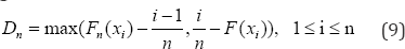
Where, D_n is the K-S distance; n is total number of data points; F(x) is distribution function of the fitted distribution; F_n(x) equals to i'/n; i is the cumulative rank of the data point. There are two hypothesises that are the null hypothesis (H₀) and the alternative hypothesis (HJ in the K-S test. H₀ assumes that the data follows a specified distribution, and the H does not. The fixed values at a chosen significance level (α), e.g. 0.01, are generally used to evaluate H₀. If the test statistic D is greater than the critical value obtained from a table, the hypothesis concerning the distributional form is rejected at α.

Results

The data subsets classified grade bins and time of day are then been tested for the generalized logistic distribution and Wake by distribution. Comparisons between Histograms of the empirical data and fitted curves are illustrated in Figure 1 through 3 by time-of-day. In addition, P-P plots provide the magnification of differences of sample and model distributions are presented to the same dataset on these three figures. Figures 1-3 show the model PDF over sample histograms together with the P-P plots side-by-side of AM, mid-day, and PM data, respectively. There is very distinguishing characteristics of VSP distribution that almost every histogram has a peak. From the AM and PM GPS data distributions (as shown in Figures 1 & 3, respectively), it is found that the Wake by distribution fits the samples very good at smaller grades and the differences between sample and model distribution grow with the increase in the grade, especially at greater than 10% and less than -10%.

For the mid- day datasets, the Wake by distribution does not fit best for smaller grades including 0 to 2%, 2% to 4%, -2% to 0 and -4% to -2% bins. Instead, the generalized logistic distribution fits the data better and the P-P plots are almost perfect straight lines. Comparing to the fit from mid- day datasets as shown in Figure 2, more noise was observed on the comparison of histograms and PDF and the P-P plots of the peak-hour datasets in Figures 1 & 3. This noise maybe introduced by the relevantly large speed variations during peak hours. K-S test results show that all samples follow a specific distribution; therefore the entire null hypothesis is accepted. Consequently, the selection of fitted distribution is based on the comparisons of PDFs, P-P plots and the K-S tests. The fitted parameters by grade and time of day are listed in Table 2.

Conclusion and Future Research

from the study site fit into a specific distribution function, i.e. the generalized logistic or Wake by distribution, which is expected The paper presents an approach to incorporate freeway to use the function to determine the MOVES operating mode grade into the current VSP profiling study. Samples collected distribution empirically for emission and energy consumption modelling. The findings of this research can be summarized into the following:

a. There is a strong connection between VSP distribution and freeway grade.

b. The sample distribution of VSP can be well presented at lower grade bins such as -4% to 4%. However, the goodness of fit declines when the grade increases or decrease to a larger number.

c. Wake by distribution is able to capture most distribution characteristics of VSP at all grade bins in a higher speed variation traffic condition, while, the generalized logistic distribution fits the sample data better at smaller grade bins ranging between -4% and 4%when there is less variation in vehicle speeds.

d. The speed variation plays an important role in determining the VSP distribution. Larger speed variation corresponding to more congested traffic results in a less randomized distribution.

e. The speed variation is a contributing factor distinguishing the distributions of AM, PM and Mid-day datasets.

The current practice in mobile source emissions modelling suggests significance of using second-by-second vehicle operation data to generate an accurate estimate of emissions for the transportation network. A better understanding and profiling of vehicle VSP distribution provided by the paper can certainly help to obtain more accurate modelling results. In addition, the findings provide good references for preparing operating mode distribution inputs for the MOVES model, since the distribution function can be used to generate and validate simulation results, the study. For our future research, it would be interesting to examine the grade-specific VSP distributions for other roadway types, such as arterials and local streets. In addition, correlating the emission rates with grade-specific VSP distributions would be an improvement to our study and vehicle emission and consumption modelling.

 

For more articles in Open Access Journal of Environmental Sciences & Natural Resources please click on: https://juniperpublishers.com/ijesnr/index.php